A reader wrote :
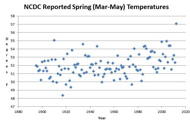
This got me interested to see what USHCN was doing to springtime temperatures. The graph below is what NCDC reports.
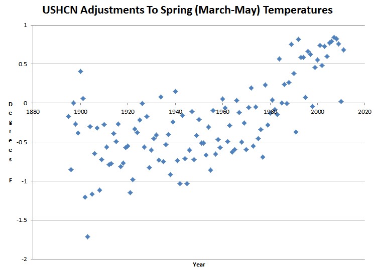
So I calculated the adjustments they did through 2011 vs. the raw daily data. Stunning indeed! They added about two degrees on to recent temperatures relative to 100 years ago.
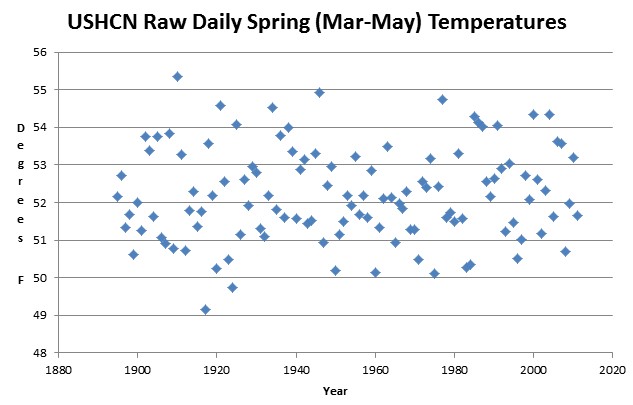
The spring of 1934 was probably just a warm as spring 2012, but the data has been so severely altered, that the NCDC graphs are meaningless garbage
The raw graph (calculated from daily data) is shown below. 2012 is not included because that data is not available yet.
Note the similarity between the adjustment graph, and Hansen’s temperature graph in the article below this one.
Raw data below :
Year	Daily Raw	NCDC	Adjustment
1895	52.16933333	52	-0.169333333
1896	52.71106667	51.86	-0.851066667
1897	51.32856667	51.33	0.001433333
1898	51.68836667	51.42	-0.268366667
1899	50.62173333	50.24	-0.381733333
1900	52.01113333	52.42	0.408866667
1901	51.263	        51.32	0.057
1902	53.75673333	52.55	-1.206733333
1903	53.3941	        51.68	-1.7141
1904	51.63103333	51.33	-0.301033333
1905	53.7593	        52.59	-1.1693
1906	51.07523333	50.43	-0.645233333
1907	50.89956667	50.58	-0.319566667
1908	53.82733333	52.71	-1.117333333
1909	50.78736667	50.06	-0.727366667
1910	55.3474	        55.07	-0.2774
1911	53.26366667	52.7	-0.563666667
1912	50.71096667	49.92	-0.790966667
1913	51.78576667	51.01	-0.775766667
1914	52.3006	        51.91	-0.3906
1915	51.35383333	50.86	-0.493833333
1916	51.74836667	51.48	-0.268366667
1917	49.16276667	48.35	-0.812766667
1918	53.56833333	52.8	-0.768333333
1919	52.1783	        51.61	-0.5683
1920	50.24296667	49.69	-0.552966667
1921	54.57816667	53.43	-1.148166667
1922	52.5525	        51.57	-0.9825
1923	50.47273333	50.14	-0.332733333
1924	49.72783333	49.35	-0.377833333
1925	54.07786667	53.86	-0.217866667
1926	51.1473	        51.14	-0.0073
1927	52.6126	        52.05	-0.5626
1928	51.92136667	51.75	-0.171366667
1929	52.94486667	52.12	-0.824866667
1930	52.81023333	52.21	-0.600233333
1931	51.30533333	50.85	-0.455333333
1932	51.0973	        50.69	-0.4073
1933	52.18916667	51.46	-0.729166667
1934	54.5217	        54.6	0.0783
1935	51.81783333	51.07	-0.747833333
1936	53.77023333	53.24	-0.530233333
1937	51.59523333	51.19	-0.405233333
1938	54.00566667	53.09	-0.915666667
1939	53.35303333	53.11	-0.243033333
1940	51.57216667	51.72	0.147833333
1941	52.88563333	52.15	-0.735633333
1942	53.13206667	52.1	-1.032066667
1943	51.45186667	51.29	-0.161866667
1944	51.50893333	50.8	-0.708933333
1945	53.29183333	52.26	-1.031833333
1946	54.91286667	54.31	-0.602866667
1947	50.94503333	50.84	-0.105033333
1948	52.44356667	51.72	-0.723566667
1949	52.9447	        52.53	-0.4147
1950	50.1998	        49.99	-0.2098
1951	51.1512	        50.64	-0.5112
1952	51.4912	        50.98	-0.5112
1953	52.17936667	51.51	-0.669366667
1954	51.9088	        51.6	-0.3088
1955	53.211	        52.35	-0.861
1956	51.67593333	51.58	-0.095933333
1957	52.18553333	51.53	-0.655533333
1958	51.59763333	51.13	-0.467633333
1959	52.86053333	52.29	-0.570533333
1960	50.13736667	50.19	0.052633333
1961	51.33943333	51.28	-0.059433333
1962	52.10013333	51.61	-0.490133333
1963	53.47796667	53.19	-0.287966667
1964	52.12756667	51.5	-0.627566667
1965	50.9459	        50.35	-0.5959
1966	51.96773333	52	0.032266667
1967	51.85066667	51.73	-0.120666667
1968	52.29246667	51.79	-0.502466667
1969	51.2744	        51.02	-0.2544
1970	51.27506667	50.68	-0.595066667
1971	50.4837	        50.43	-0.0537
1972	52.5636	        52.76	0.1964
1973	52.39073333	51.84	-0.550733333
1974	53.15883333	53.11	-0.048833333
1975	50.12253333	49.67	-0.452533333
1976	52.4377	        52.1	-0.3377
1977	54.73486667	54.04	-0.694866667
1978	51.60426667	51.84	0.235733333
1979	51.74223333	51.46	-0.282233333
1980	51.49796667	51.37	-0.127966667
1981	53.30816667	53.35	0.041833333
1982	51.5623	        51.48	-0.0823
1983	50.2756	        50.13	-0.1456
1984	50.35533333	50.92	0.564666667
1985	54.29673333	54.3	0.003266667
1986	54.12783333	54.37	0.242166667
1987	54.02363333	54.02	-0.003633333
1988	52.56606667	52.83	0.263933333
1989	52.16696667	52.92	0.753033333
1990	52.6262	        53.01	0.3838
1991	54.05136667	53.68	-0.371366667
1992	52.9149	        53.73	0.8151
1993	51.21626667	51.8	0.583733333
1994	53.02523333	53.61	0.584766667
1995	51.45953333	51.53	0.070466667
1996	50.50443333	51.17	0.665566667
1997	51.0173	        51.64	0.6227
1998	52.7064	        52.66	-0.0464
1999	52.0749	        52.53	0.4551
2000	54.3281	        54.88	0.5519
2001	52.62233333	53.36	0.737666667
2002	51.1756	        51.66	0.4844
2003	52.3108	        53.04	0.7292
2004	54.35183333	54.95	0.598166667
2005	51.61603333	52.39	0.773966667
2006	53.61003333	54.4	0.789966667
2007	53.5653	        54.41	0.8447
2008	50.6838	        51.51	0.8262
2009	51.97833333	52.74	0.761666667
2010	53.19943333	53.22	0.020566667
2011	51.66026667	52.34	0.679733333


Woah! 0.37°F of warming in 2°F of adjustments? I’m dying of heat prostration here.
AGW… Alarmists Gone Wild!!!!!
Spring break may be over in Rio, but that does not mean that the party is over… watch as crazed ‘climate experts’ heat up the airwaves with hotter than ever predictions of a sizzling doomsday!
Has anyone tried to explain the justification for the adjustments? Or is it just blatant cheating?
Have not read anything about why the adjustments are made, but it does appear that the claim that adjustments in recent years are nearly always up and in years in the early part of the century, they are down. I think that looks kind of like blatant cheating…….
Stephen and readers,
All of the data, as well as a description of the corrections for known inhomogeneities, are available at the link below.
http://lwf.ncdc.noaa.gov/oa/climate/research/ushcn/ushcn.html#QUAL
The cumulative effect of the adjustments for Time of Observation Bias, MMTS/CRS bias, and
Urban Heat Island effects is a gradual 0.5F warming since around 1970. Earlier years have not been significantly affected by these adjustments. See the graphic of Raw USHCN – Adjusted USHCN here: http://lwf.ncdc.noaa.gov/img/climate/research/ushcn/ts.ushcn_anom25_diffs_urb-raw_pg.gif.
Time of Observation Bias was a correction to a known inhomogeneity caused by the earlier practice of setting the min/max thermometer in the late afternoon or evening. On days when, for instance, a cold front would pass or the following day would be cloudy and rainy, the high would be recorded as the set maximum from the previous day. The adjustment is rather small — only a few tenths of a degree — and based on sound science.
The correction for MMTS was due to the switch from cotton region shelters to MMTS. It was discovered that the MMTS sites had a slight cool bias compared to the the cotton region shelters. This correction is designed to eliminate the cooling bias imparted by the switch to MMTS, and again is based on sound, published scientific methods.
The correction for UHI is minimal, and is based on a regression analysis comparing sites affected by urbanization to nearby non-urban sites. This correction is minimal, and I believe generally a negative correction. For some sites that have moved from city centers to the outskirts of the city (most sites haven’t moved that much, but they may if it’s a data sparse region), the UHI correction may actually be slightly positive to correct for step changes associated with the site move. The overall effect, however, is minimal.
The net of these effects, again, is rather small. Only on the order of an effective warming of about 0.5F in recent years, and are only designed to eliminate KNOWN biases in the data set. For comparison, Spring 2012 was about two degrees warmer than the previous record. Even eliminating these adjustments, it would still be about 1.5 degrees warmer than the previous record. Moreover, the effect on the reported trend is probably only on the order of a couple tenths of a degree, out of a trend of about +1.2/century. Given the U.S. is only about 0.02% of the earth’s surface, these changes would affect the reported global trend to the extent of maybe a tiny fraction of a hundredth of a degree.
The “apparent” downward adjustment Stephen found in earlier years is because he merely took the average of all of the data points without correcting for geographic distribution. Obviously, if the geographic distribution of the sites has changed you have to adjust accordingly.
Hope this helps!
Complete BS.
You are looking at USHCN1 documentation which is now obsolete for a decade. The USHCN2 adjustments are about 3X that size..
USHCN stations tend to be fairly evenly distributed geographically, and the same patterns of adjustment are seen in the state by state data, which makes your point completely moot.
Computers are very efficient tools for generating large amounts of meaningless data. The fact that someone implemented some flaky algorithms in software is not particularly impressive
The 1.5 degree adjustments are larger than the claimed trend. which means a signal to noise ratio of less than one. That is what you call sound science? It is junk science at its worst.
The “apparent” downward adjustment Stephen found in earlier years is because he merely took the average of all of the data points without correcting for geographic distribution. Obviously, if the geographic distribution of the sites has changed you have to adjust accordingly.
This argument has been used before, but does not stand up under scrutiny, as this analysis in Alabama shows.
http://notalotofpeopleknowthat.wordpress.com/2012/06/08/ncdc-cooling-the-past-again/
Why is a “couple of tenths of a degree” insignificant when adjusting data but HUGE on those warming graphs? If .2 of a degree is not a big deal, why are all warming graphs done in .10 increments. Because it IS significant when you want it to be and not if you don’t.