
Climate science has gone 100% veracity free. Desperate to keep their scam funding alive, there seems to be no limit on how dishonest scientists will get.
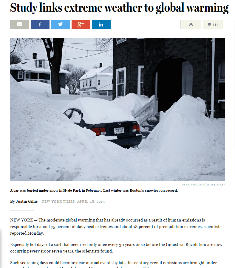
New study finds strong link between weather extremes, global warming – Nation – The Boston Globe‘
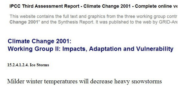
Flagrant lies. The IPCC predicted mild winters and less snow
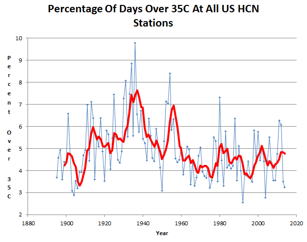
The frequency of hot days has plummeted over much of the world. In the US, hot days are much less common than they were 80 years ago.
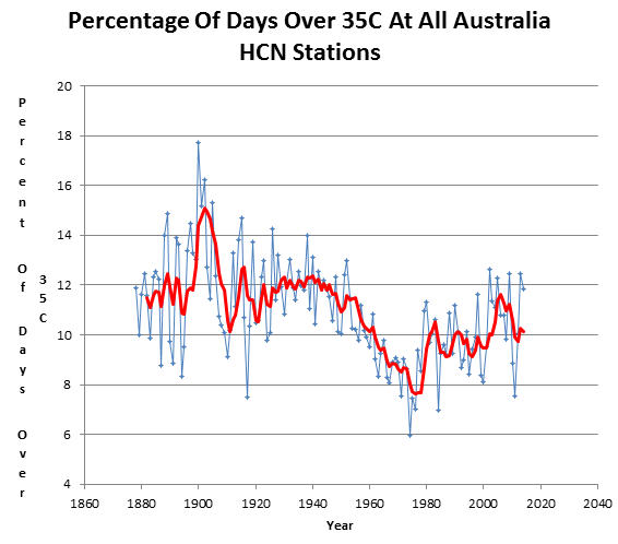
Hot days in Australia are much less common than they were at the start of the 20th century.
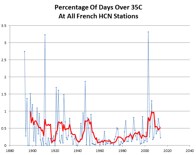
Hot days in France were more common at the end of the 19th century.
These 100% fraudulent studies are becoming increasingly common, as scientists become increasingly desperate to keep their scam alive.

And it only took 25 different models to arrive at this delusion.
Fools ignore complexity. Pragmatists suffer it. Some can avoid it. Geniuses remove it.
-Alan Perlis
It is always amazing how the so-called “climate scientists” will make some models — which we know are not able to represent the atmosphere on a fine enough scale (for example http://climateaudit.org/2005/12/22/gcms-and-the-navier-stokes-equations/ ) — look at the results and proclaim a definitive statement about forthcoming global doom.
Imagine this analogous situation:
“”I can prove that CAGW is a scam!”
“Really? How?”
“Well, I wrote three novels about the subject, and in all three it was revealed at the end that the climate scientists were altering the data!”
“What?!! Three NOVELS! How does that prove anything? You know that they are fiction, right?”
“Well, sure! Of course they are fiction — but it is very realistic fiction! I made them as believable as I could.”
“Being realistic is nice, but just because something is realistic, that does not make it actual reality. You can’t prove something by making up a story about it!”
“Normally, I would agree with you. But I wrote all three of these novels using a word editing program. Using a computer to write them make the stories become real!”
“I’ve never heard anything so crazy!”
“I have…”
🙂
It is not only the Unknown Unkowns but the studiously ignored Knowns that are going to bite the ClimAstrologists in the arse.
Now if we could some how aim the inner city types at the universities, the ensuing destruction would improve society.
A wee bit of Karma — ‘Reap what you sow’ would be really nice.
https://media2.stickersmalin.com/produit/100/stickers-devil-smile-R1-143760-2.png
I would just like the modelers to list all climate forcings, order them from most to least effective, and then quantify them.
After all, it is “settled science”.
Gator,
Shirley you Jest.
“Why should I give you my data when all you want to do is find something wrong with it?” — Phil Jones
That cheered me up on this cold miserable morning 😉
Professor Bigsley really blew it when he picked Boston MA as his first test case.
http://conservatoons.deviantart.com/art/Stupid-Detector-97612450
http://fc04.deviantart.net/fs36/f/2008/254/3/f/Stupid_Detector_by_Conservatoons.jpg
Shouldn’t that be:
Professor Bigsley STUPIDly turns onn his new Stupidity Detector when a Global Warming seminar/tent revival is in town.
?
That way you underscore the idea of a positive feedback
What are their choices? If the say nothing, the facts crush them, and thet lose their grants.
if they lie, they postpone the day of reckoning. If they tell the truth, they not only lose
their grants, they may be liable to refund the grants, and go to jail
Perhaps they are hoping to retire before it is too late. They plan to move to a tropical place close to the sea and preferably with no extradition treaty with the USA. Then when the wheels fall off the AGW cart, they imagine they will be safely out of reach of both US law and the coming Ice Age.
Occam’s Razor would say that big yellow circle in the sky might be the most important.
If you pay someone to prove A+B=C, C will always be the answer you get.
The IPCC charter…
“ … to assess on a comprehensive, objective, open and transparent basis the scientific, technical and socio-economic information relevant to understanding the scientific basis of risk of human-induced climate change, its potential impacts and options for adaptation and mitigation. IPCC reports should be neutral with respect to policy.“
It was a hit job from the start, a prosecution and not an investigation.
The human species was found guilty before the trial and the MSM has been stirring up the lynch mob. Only problem is the lynch mob has not realized it is themselves they are murdering.
Sort of reminds me of the inner city types burning their own supply lines — Go figure.
https://www.youtube.com/watch?v=WHavrNx5eO0
The new bullshit is this 75% Garbage…
75% of extreme weather caused by .0004 mole CO2… laughable… were it not so serious…
Let’s discuss ppm.
The IGSS site (Mass of atmos CO2 page) says ppm is volumetric based. I have seen other sources that refer to ppm as volumetric based including references to Mauna Loa. ppmv
Another approach has ppm that is gram weight based. ppmgw
World Bank 4C report says ppm is mole based. ppmmol
Which is it? Which one did IPCC use? Why don’t they specify?
Since the specific volume of CO2 is less than that of air, the anthro CO2 ppm volumetric or mole basis will be even less than the gram weight based. All of these cases use the residual 45% atmospheric component.
IPCC AR5
Year……ppm
1750……278
2011……390.5
Diff…….112.5
Additional CO2 due to man…….555 PgC, 375 PgC due to fossil fuel and cement production.
ppm gram weight based=(grams CO2 added)/(atmospheric grams)
(3.75E+17/ 5.14E+21)*.45 = 32.8 ppm or about 30% of the 112.5 ppm CO2 increase between 1750 and 2011.
ppm volumetric based=((grams CO2 added)/((1.842 grams CO2)/m^3 ))/((grams air)/((1.205 grams air)/m^3 ))
(3.75E+17 * 1.205)/ (5.14E+21 * 1.842)*.45 = 21.6 ppm or about 21.6% of the 112.5 ppm CO2 increase between 1750 and 2011.
ppm mole based=((grams CO2 added)/((44.01 grams CO2)/mole))/((grams air)/((28.97 grams air)/mole))
(3.75E+17 * 28.97)/ (5.14E+21 * 44.01)*.45 = 21.5 ppm or about 21.5% of the 112.5 ppm CO2 increase between 1750 and 2011.
Mankind’s fossil fuel and cement CO2 production contributed about 21.5% of the CO2 ppm increase between 1750 and 2011.
There is more to this issue…
The notion of low pre-industrial CO2 atmospheric level, based on such poor knowledge, became a widely accepted Holy Grail of climate warming models. The modelers ignored the evidence from direct measurements of CO2 in atmospheric air indicating that in 19th century its average concentration was 335 ppmv (Figure 2). In Figure 2 encircled values show a biased selection of data used to demonstrate that in 19th century atmosphere the CO2 level was 292 ppmv. A study of stomatal frequency in fossil leaves from Holocene lake deposits in Denmark, showing that 9400 years ago CO2 atmospheric level was 333 ppmv, and 9600 years ago 348 ppmv, falsify the concept of stabilized and low CO2 air concentration until the advent of industrial revolution.
-Prof. Zbigniew Jaworowski
Chairman, Scientific Council of Central Laboratory for Radiological Protection
Warsaw, Poland
http://www.warwickhughes.com/icecore/call2.jpg
http://www.john-daly.com/zjiceco2.htm
More Cherries. Surprise!
Dag, nabbit Gator, you type faster…
Barrow Alaska CO2 data for 1947-1948 data shows 420 ppm! (average of 330 samples) It is noted that the Keeling samples (1972 to 2004) are transported from Barrow Alaska to California before they are analysed. (wwwDOT)biokurs.de/eike/daten/leiden26607/leiden6e.htm
Here is Becks information from Barrow:
Date – –Co2 ppm * * latitude * * longitude * * *author * * location
1947.7500 – – 407.9 * * *71.00* * * -156.80 * * *Scholander * *Barrow
1947.8334 – – 420.6 * * *71.00* * * -156.80 * * *Scholander * *Barrow
1947.9166 – – 412.1 * * *71.00* * * -156.80 * * *Scholander * *Barrow
1948.0000 – – 385.7 * * *71.00* * * -156.80 * * *Scholander * *Barrow
1948.0834 – – 424.4 * * *71.00* * * -156.80 * * *Scholander * *Barrow
1948.1666 – – 452.3 * * *71.00* * * -156.80 * * *Scholander * *Barrow
1948.2500 – – 448.3 * * *71.00* * * -156.80 * * *Scholander * *Barrow
1948.3334 – – 429.3 * * *71.00* * * -156.80 * * *Scholander * *Barrow
1948.4166 – – 394.3 * * *71.00* * * -156.80 * * *Scholander * *Barrow
1948.5000 – – 386.7 * * *71.00* * * -156.80 * * *Scholander * *Barrow
1948.5834 – – 398.3 * * *71.00* * * -156.80 * * *Scholander * *Barrow
1948.6667 – – 414.5 * * *71.00* * * -156.80 * * *Scholander * *Barrow
1948.9166 – – 500.0 * * * * *71.00* * * -156.80 * * *Scholander * *Barrow
These data must not be used for commercial purposes or gain in any way, you should observe the conventions of academic citation in a version of the following form: [Ernst-Georg Beck, real history of CO2 gas analysis, (wwwDOT)biomind.de/realCO2/data.htm ]
Scholander got more than a 100ppm swing at Barrow over a year’s time.
http://www.greenworldtrust.org.uk/Science/Images/ice-HS/Fig-1.gif
http://www.greenworldtrust.org.uk/Science/Images/ice-HS/fonselius-detail.gif
Atmospheric CO2 and Global Warming: A Critical Review
Historic variations in CO2 measurements
Of interest:
Were key 1995 IPCC scientists’ conclusions of man-made global warming, tampered with?
The measurement techniques were probably accurate back then (1860-1960) but the samples were likely contaminated. Today, more care is taken to obtain a “good” sample and the analytical techniques have better precision and accuracy (in general). There is no physical mechanism by which earth’s atmospheric CO2 could vary by 100 ppm or more in a very short period of time (1 or 2 years), which the early data shows. This indicates that the early results do not accurately measure global atmospheric CO2.
You are making the assumption that CO2 is uniform in the atmosphere. An idiotic assumption without a lot of proof since there are numorous sources and since and CO2 is heavier than air. I have been round and round on this assumption with F. Englebeen but I do not have all my various data to hand.
One bit of information is the satelites show the CO2 is not uniform despite the sample size being in the range of kilometers^2 (^3?) (Don’t have the URL)
https://chiefio.files.wordpress.com/2013/01/jaxa-xco2_l2_201208010831average_v02_11.png
Dr. Glassman also addresses the issue:
Correct Gail, and besides, Prof Zbigniew Jaworowski is not an idiot.
Nor is Dr Glassman or Dr Segalstad http://www.co2web.info/
Of course the atmosphere is not homogenous, however, it’s closer to being well mixed than not. We all know that there are sources and sinks. In the olden days it was more difficult to get to pristine environments not influenced by local sources, whether these be a burning fire or even ones breath. It would be a bad idea to measure CO2 indoors or near a factory and use that measurement to represent global CO2 concentration.
CO2 is heavier than N2 or O2 but eventually, these diffuse into each other (diffusion is entropy driven). On average, the concentration globally is going to be within +/- 10 ppm of the mean. We can’t go back in time and no one intentionally took representative samples of the atmosphere for future measurements of CO2. However, the scatter of the old data indicates that there was a sampling problem back then. That data cannot be dismissed entirely, but objectively we can see that the scatter is indicative of poor precision.
https://www.youtube.com/watch?v=x1SgmFa0r04
R. Shearer says: ….CO2 is heavier than N2 or O2 but eventually, these diffuse into each other (diffusion is entropy driven). On average, the concentration globally is going to be within +/- 10 ppm of the mean….
It is the “eventually” that is the I Gottcha!
“The CO2 concentration at 2 m above the crop was found to be fairly constant during the daylight hours on single days or from day-to-day throughout the growing season ranging from about 310 to 320 p.p.m. Nocturnal values were more variable and were between 10 and 200 p.p.m. higher than the daytime values.” http://www.sciencedirect.com/science/article/pii/0002157173900034
The extreme lower limit of 200 ppm can also be found in green house studies:
The sources and sinks plus Carbon dioxide is heavier than air and does not easily mix into the greenhouse atmosphere by diffusion means Co2 is NOT going to be well mixed.
MORE ON WELL MIXED”
The sequestration rates of CO2 are dependent on partial pressure. High local atmospheric concentrations induce high local sequestration. And consideration of seasonal variations in atmospheric CO2 at a variety of locations indicates that most locally released CO2 (from any source, natural or anthropogenic) is sequestered locally
(ref. Rorsch A, Courtney RS & Thoenes D, ‘The Interaction of Climate Change and the Carbon Dioxide Cycle’ E&E v16no2 (2005) ).
You see more than 80 ppm variation in Harvard forest. From 320 ppm to around 420 ppm with a set of outliers to 500 ppm.
There is no excuse for Manua Loa Obs for tossing out a lot of data.
The annual mean CO2 level as reported from Mauna Loa
CO2 is released by the Mauna Loa and the adjacent Kilauea volcanoes. This volcanic CO2 is
(a) driven aloft by the sea breeze by day, and
(b) driven back down by the land breeze at night.
Hence, it is a gross and improbable assumption that these volcanic emissions do not significantly affect the measurement results
Is this the description of true, unbiased research? The assumption is made that there is NO VARIABLITY and the data is adjusted to reflect that!
I tried to dig up the AIRS data. Might notes show:
CO2 nadir resolution of 90 km X 90 km.
http://airs.jpl.nasa.gov/data/about_airs_co2_data/
Unfortunately it now returns page not found.
However googling for : AIRS CO2 nadir resolution of 90 km X 90 km.
Returns:
http://disc.sci.gsfc.nasa.gov/AIRS/documentation/v5_docs/AIRS_V5_Release_use_Docs/AIRS-V5-Tropospheric-CO2-Products. pdf
Gives page not found or it just keeps looking. This is typical of ‘inconvienent’ information. It vanishes off the internet.
Here is the AIRS july 2008 CO2 (ppmv) map:
http://photojournal.jpl.nasa.gov/jpegMod/PIA11194_modest.jpg
Plants can be both a source and sink for CO2 (mostly a sink due to photosynthesis). No argument here. In fact that represents the issue that is in essence what I am trying to communicate. And yes, cold water absorbs more CO2 and warm water less.
I did not say that CO2 was uniform, I clearly said that it was not homogenous although on average (average being the sum of the measurements divided by number of measurements) is within +/- 10 ppm (globally). As I said, one should be careful in measuring CO2 at any one point and then extrapolating that measurement to represent a “global” concentration. It’s very similar to temperature measurements and fraught with many of the same issues.
Now one might think that measuring CO2 on the top of a volcano is a crazy thing to do, but the measurement method takes advantage of natural air circulation to avoid contamination and the results give a good representation of pristine air in the middle of the Pacific. The measurement method is precise enough to show the annual variation due to plant respiration. My point is that the measurements made by the best methods in the 1800s-1900s were not precise enough to show this. They were in fact inaccurate and had scatter of over 100 ppm in some cases. It is perfectly valid to throw out results that are obtained from contaminated samples or from methods that are inaccurate and or in precise.
NOAA actually has a network of stations throughout the world. The measurements are of high quality, much better than in the past and the trends that they produce are more reliable. In chemistry, we speak of experimental error. The experimental error today is much lower.
R. Shearer,
You are saying that the Keeling measurements taken at Mauna Loa are more accurate.
Again I disagree.
It is too late to dig up the exact reference, however Dr. Jaworowski and Dr Segalstad said that Keeling used a newly developed insturment, an Infrared Spectrophotometer (dual beam) and he never did the validation studies. This was in the 1960-1970s.
As it happened Perkin-Elmer was advertising their Infrared Spectrophotometer as being able to do quantitative analysis. At the time my Lab was using a Gas Chromatograph and the method took a really long time so we bought a new IR and I was the one who was supposed to develop a new test method.
In a word the IR SUCKED! I could not get any decent repeatablity. It was great for identification but we never were able to get it to work as an analytical tool.
No wonder Mauna Loa tosses out the ‘outliers’!
Ernest Beck did the error analysis:
http://www.biomind.de/realCO2/bilder/CO2back1826-1960eorevk.jpg
FROM: http://www.biomind.de/realCO2/
Gail, you were using GC to measure CO2? What detector?
When Keeling began his work, GCs were not even commercially available. CO2 is actually a good infrared absorber, kind of goes without saying, and IR spectroscopy is actually a good technique for CO2 in air.
Back in the 1800’s, it was worse. No IR, no GC, yes, scales were good but no standards, such as ISO or ASTM. Few commercially prepared reagents with validated spec sheets. The data generated back then was of high quality for the time and the chemists were good but there was no Aldrich Chemical company.
Ernst Beck did a good error analysis and what I am saying is consistent with his work. Look at the error bars! Are you saying the measurements are not becoming better? If you are, then you are saying the opposite of what Beck is.
http://oco.jpl.nasa.gov/images/ocov2/1stmap.jpeg
Better representation of the global CO2 contributors than the NASA video.
“cold water absorbs more CO2 and warm water less.”
https://youtu.be/wK4reyh86w0
“Mankind’s fossil fuel and cement CO2 production contributed about 21.5% of the CO2 ppm ”
MORE PLEASE , says the world’s biosphere.
CO2 is one of the 2 main building blocks for ALL life on this Earth, and has been too low for a long. long time.. That is the REALITY, Nick.
The CO2 man’s fossil fuel & cement production (IPCC’s category) put in the atmosphere between 1750 and 2011 increased the atmospheric CO2 level by about 5.5%. Doesn’t look like a dangerous trend to me. Evaporating water vapor soaks up any additional CO2 “downwelling” perpetual motion heating anyway.
So what problem does shutting down coal and installing green power solve except financing the green industry and government grant business?
Too many humans cluttering up the USA and the EU….
As you can see from your calculations, ppm mol and vol are equivalent. Per the ideal gas equation (PV=nRT) volume and mole fraction are additive (P is fixed and R is a constant). Using mass in this case does not make sense to do since mass is not constant with changing composition.
Yes, I discovered that ppm gram basis was the wrong way to go. But why don’t all these papers and IPCC spell out what they are using? And how?
And if it’s carbon as carbon say PtgC or GtC and if it’s carbon as carbon dioxide say so with PtgCO2 or GtCO2?
Lazy? Imprecise? Deceitful? Obfuscating on purpose?
As Gail and others above point out, referring to CO2 as “carbon” is intentionally being deceptive. On the other hand, there is merit to accounting for a “carbon” balance on an elemental basis.
With regard to ppm units, chemists doing work with gaseous samples understand that ppmv and ppm mol are equivalent and frequently just use “ppm.” Similarly for water analysis ppm is used but it is understood to mean ppm mass or mg/L, which happens to be equivalent at least for solutions that have a density close to 1 g/mL. Everybody is lazy at some point, though.
Climate Hoax logic:
If it’s bad weather (read; incnvenient for people) it must be caused by humans because the weather as if guided by some divine Michael Mann in the sky would always be perfect for everyone at all times.
During the Little Ice Age, everyone thought witches were changing the weather.
Now they think it is those EVIL ‘Climate Change Deniers’ and some are calling for our death. And so we enter the next Dark Ages…
Now Catalina Island is sinking (maybe) or rising (who knows) but a new study by Stanford shows that the Island could be underwater in 3 million years!
Catalina Island will be somewhere around Anchorage, Alaska by then.
Actually, the last IPCC report stated it is not possible, at present, to link increases in extent or amount of any extreme weather to global warming.
—-and here we have an inconsistency. One cause of more extremes in weather events would be a larger gradient in temp from the equator to the poles. This increase would cause a larger difference in pressure areas causing more violent winds. So, if there were more warming at the poles, as alarmists predict, there would be a tendency for less extreme weather. I think the IPCC circle has had to consider this in their statements
Secondly, a fundamental outcome of an increase in greenhouse activity, should, according to models, warm the atmosphere near the earth’s surface and cool it in higher altitudes. This difference should be greater near the equator where the surface of the earth has the highest percentage of water. However, the predicted equatorial ‘hot spot’ has not happened.
The larger vertical temperature would cause more convective forces causing more violent weather.
This, also, has not happened. Another modeled prediction not confirmed by observation!
Maybe we can have a contest as to who can list the most failed predictions
Maybe, I will give in to Gail already.
snicker
https://media2.stickersmalin.com/produit/100/stickers-devil-smile-R1-143760-2.png
Gator and I would probably tie.
https://www.youtube.com/watch?v=9vdl3TRxv0c
I just wonder why they still show steam or particulate smoke as CO2
CO2 is an invisible life building gas.
To scare the low information dummies.
It is why they call it carbon to equate it with soot. That is why people think it is a polutant. Even those who realize it is a gas think it is carbon MONOXIDE and not Carbon DIOXIDE.
Catchy tune. We should make this the National anthem. I forgot who first posted this video here this last week.
If it weren’t so sad, the swings between “settled science” and “a new study shows” would be hilarious.
The science is settled. The debate is over. 97% of the media is just a bad joke on the public. http://www.globalcoolingcausesglobalwarming.blogspot.com
Earthquake sun connection
http://cafe368.daum.net/_c21_/bbs_search_read?grpid=1FBty&fldid=N0WJ&datanum=1898&contentval=&docid=1FBtyN0WJ189820100616141523
Solar -Volcanic Activity connection
http://adsabs.harvard.edu/full/2003ESASP.535..393S
(use entire string including ..393S)
or click link
link
IPCC uses heads I win, tails you lose logic.
For seventy years, society faced two major puzzles:
1. Why was there a news blackout of major events in Aug-Sept 1945?
2. Why did mainstream consensus scientists hide, ignore or adjust data that falsified their models?
We now know one answer explains both puzzles: STALIN WON WWII:
https://dl.dropboxusercontent.com/u/10640850/Temperature_Data.pdf
R. Shearer says: “Gail, you were using GC to measure CO2? What detector?
When Keeling began his work, GCs were not even commercially available. CO2 is actually a good infrared absorber, kind of goes without saying, and IR spectroscopy is actually a good technique for CO2 in air…..”
…….
I was using GCs in 1968 and IRs in 1973. I was analysing organic drug precurors (FDA AUDITS!!!) They had strong IR absorption but the machine response was all over the place. Back then we wer using a ruler to define a triangle that approximated the area under the curve for both machines. The GC was good to parts per million even with that method. The IR was pure crap.
On Keeling and Callendar and their fudging of data:
This is a different paper by Dr Segalstad
I recommend reading both in full.
If said drug precursors were solids, then you probably had to press them into an IR transparent pellet for analysis. Certainly, IR is better for some applications than others. CO2 absorbs very nicely at 1750 nm and in the case of CO2 in air, a gas cell requires no such sample pretreatment and can be of large volume (so more molecules in the IR beam’s path).
In any case, I think you would have to agree that modern computers that integrate automatically and obviate the need manual triangulation are better for both precision and accuracy as well as ease of automation.
I agree with you that is was possible to make good measurements by physical means, titration, prior to instrumental methods. On the other hand measurements that show 550 ppm one year and 300 ppm the next year do not look good and that is what the early record shows. Given that bad data exists, climate scientists so inclined will tarnish good data with the bad. Convincing anyone of the validity of the early work is a hard sell.
I’ve analyzed CO2 in air using mass spectrometry, for calibration purposes, not for the purpose of quantifying it. I think that NOAA actually accounts for the difficulties quite well and as I noted previously, Mauna Loa is one of only many stations, but for some reason is the one that everyone wants visit :).
I want to second Gail here, at least with respect to GCs and IR spectroscopy as it was back in the 60s/70s. I’m a bit younger, but we used ‘antique’ machines all of the time. We preferred GC/MS for ‘precise = high resolution’ work. IR spec was too flaky. The machine we had was so flaky only one person was allowed to run it (which complicated doing error analysis, since you could not be certain of what the operator did and if you cited operator error in other than the most general terms you had a political problem).
My chemistry pedantry meter pegs when people talk about carbon dioxide being heavier than air. Okay, yes; but for gases at surface temperatures and pressures the molecules are moving quickly and randomly. What you can say is that carbon dioxide molecular diffusion speed is slower than oxygen (which is also technically heavier than air) or nitrogen or argon. This allows one to seque into ‘well mixed’ Given the very large and variable sources and sinks of carbon dioxide, I think that one could only say it was well mixed if you’re talking about small volumes of air at ‘normal’ temperatures and pressures. That is a problem, to me, for the gross grid scales used by climate modelers.
And yes, 100 ppmv changes of carbon dioxide concentration is very much possible over a large enough volume with enough time and energy for chemical processes to take place, especially since these will not necessarily be uniform, even if bounded.
R. Shearer says: “…Back in the 1800’s, it was worse. No IR, no GC, yes, scales were good but no standards, such as ISO or ASTM. Few commercially prepared reagents with validated spec sheets. The data generated back then was of high quality for the time and the chemists were good but there was no Aldrich Chemical company.
Ernst Beck did a good error analysis and what I am saying is consistent with his work. Look at the error bars! Are you saying the measurements are not becoming better? If you are, then you are saying the opposite of what Beck is…..”
Why is it that the very careful work of Nobel Prize Winners get such bad press now a days?
LOOK at the Error bars again!
The error from 1880 to 1940 was LESS than the error for the time period ~1950s when Pales & Keeling were playing around with their “new infra-red (IR) absorbing instrumental method, never validated versus the accurate wet chemical techniques.”
http://www.biomind.de/realCO2/bilder/CO2back1826-1960eorevk.jpg
Also Beck matches that curve to SST (as Segalstad noted CO2 in the atmosphere is in equilibrium with the CO2 in the sea and therefore the amount is temperature dependent.)
http://www.biomind.de/realCO2/bilder/CO2-MBL1826-2008-2n-SST-3k.jpg
Fig. 2. Annual atmospheric CO2 background level from 1856 to 2008 compared to SST (Kaplan, KNMI); red line, CO2 MBL reconstruction from 1826 to 1959 (Beck 2010); CO2 1960-2008: (Mauna Loa); blue line, annual SST (Kaplan) from 1856 -2003; SST= sea surface temperature
I should have been more “precise.” The spread of the data particularly in the 1800’s is quite poor. I believe that sampling was poor and reagents and equipment was likely contaminated. A common means to dry glassware back then was to “flame” it. As we know, combustion produces CO2. It is always more difficult to measure something that is of unknown value. Of course over time analysts become more experienced and know what is real and what is an outlier. In the early days, they didn’t know that.
IR is a valid technique and is used routinely for respirometry applications in which hundreds of thousands of instruments are used today throughout the world. This paper discusses relevant history and valid for this similar application. http://www.oem.respironics.com/wp/Infrared%20Measurement%20of%20CO2%20in%20the%20Human%20Breath_Jaffe.pdf
The beastie I used was similar to this. http://antiquesci.50webs.com/PE337/IJVS6PE-2.htm
We were doing liquid samples and spiked the sample with a known amount of a chemical that did not interfere with the spectra as a calibration standard. We did ten known samples over the range in question for the initial calibration curve and then at least once a week make up three to five samples to recalibrate the curve. Unfortunately the IR just did not reproduce results as well as we would have liked in the accuracy range we were looking for.
It was a beckman double beam prism Inrared spectrophotometer purchased in 1973 and I got another one for another lab in 1977. I never had access to a computerized GC until 1985. I was just happy to have access to a hand calculator!
The PDF you linked is for human breath. An adult’s breath which contains about 35,000 to 50,000 ppm of CO2. A hundred times more CO2 then found in the atmosphere and I doubt that an accuracy of +/-2 or 3 ppm was even desired. An accuracy of 100 ppm or even 10,000 ppm would ge the monitoring job done.
……
THIS however really really bothers me and the AIRS data is handles the same way:
It is along the line of:” you will obey me, or else”
They have a preconceived notion of what the curve should be and they impose it, is my conclusion from this. Of course this is necessary with all the outgassing volcanoes in the vicinity not to mention an ocean that is changing temperature and full of green growing things.
If any data that is not within 2 standard deviations is rejected then of course you will never see swing of 80 ppm or more — it has already been edited out of the final “product”
Independent measurements?
Not hardly A while ago I managed to find a link and publications for measurements. They were all Keeling and another fellow, possibly the graduate student going through the hoops. I do not call that independent.
Here are the locations I find:
http://scrippsco2.ucsd.edu/data/atmospheric_co2.html
something like 14, and practically all the publications are Keeling et al
There is a map too
http://scrippsco2.ucsd.edu/research/atmospheric_co2.html
Keeling’s son has since taken over and all of the stations are calibrated to Mauna Loa.
So we are back to:
Here is what AIRS itself is saying:
There is no way CO2 was going to be well mixed. It was just a mythical ASSumption needed to make CAGW work It is really that simple. CAGW has always been a political whip to herd the sheeple and when you look into any of the details you find ‘adjustments’ fudging, selecting, and out right lying.
Damn, I’m sorry, I keep making a long reply and then check something and lose it. Here’s my main thing for you. If you’d like to give PE IR another go, there is a model 237 on ebay. http://www.ebay.com/itm/Perkin-Elmer-237B-Grating-Infrared-Spectrophotometer-with-Manual-/301204162952?pt=LH_DefaultDomain_0&hash=item46212ac988
Anyway, IR is a good way to measure CO2 for many applications. The breath application requires a fast response and small sample size to measure individual breaths. In the atmosphere a larger sample size and longer time constant produce greater sensitivity.
There are other many widely used IR detectors for CO2 that are validation and widely used. One you might be aware of used in pharma is the TOC analyzer. These are often capable of sub ppm sensitivity for organics in water, e.g. for cleaning validation, also required by FDA.
There are networks of other stations in other countries as well as Universities. In Colorado, we have the Mountain Research Station at Niwot Ridge. There is a common thread of standards being generated by a single group, used to be at Scripps.
More on CO2
A heck of a lot more information:
Errors in Measurements of Gas Trapped in Ancient Ice Cores.
This paper contains tons and tons of well documented information on the nitty gritty of analysing ice core samples. Well worth the read.
If there was any honesty left in science this very good, very well documented paper would have killed CAGW dead in 2007. It hits every single fallacy in CAGW and blast them with fact after fact. link
Ice core analysis represents a classic example of circular argument. Analysts continually adjusted their techniques to get the answers that they wanted. Then, some extrapolate the data to support their own conclusions.