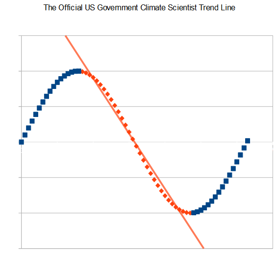
If you are a government or academic climate scientist, you can (and will) use a variant of this trend line for graphing any and all climate phenomena.
Disrupting the Borg is expensive and time consuming!
Google Search
-
Recent Posts
- Worst March Drought On Record
- ChartGL Process Control Demo
- The Biggest Money Laundering Scam
- Drought In The Headwaters Of Lake Powell
- Unrealistic Expectations Of Water Availability
- Did Bill Gates Do This?
- Worst March Drought On Record In The US
- The Real Hockey Stick Graph
- Analyzing The Western Water Crisis
- Gaslighting 1924
- “Why Do You Resist?”
- Climate Attribution Model
- Fact Checking NASA
- Fact Checking Grok
- Fact Checking The New York Times
- New Visitech Features
- Ice-Free Arctic By 2014
- Debt-Free US Treasury Forecast
- Analyzing Big City Crime (Part 2)
- Analyzing Big City Crime
- UK Migration Caused By Global Warming
- Climate Attribution In Greece
- “Brown: ’50 days to save world'”
- The Catastrophic Influence of Bovine Methane Emissions on Extraterrestrial Climate Patterns
- Posting On X
Recent Comments
- Gordon Vigurs on Worst March Drought On Record
- Robertvd on Worst March Drought On Record
- Bob G on Worst March Drought On Record
- GW on The Biggest Money Laundering Scam
- Don B on Worst March Drought On Record
- Ulric Lyons on Worst March Drought On Record
- conrad ziefle on The Biggest Money Laundering Scam
- conrad ziefle on The Biggest Money Laundering Scam
- D. Boss on The Biggest Money Laundering Scam
- Bob G on The Biggest Money Laundering Scam


Looks like you cherry picked your end points – the actual trend over the last 1.5 cycles is up.
Or maybe 1.25 cycles.
Their trend lines have direct correlation to funding levels.
Surely, that’s the Arctic ice trend line; the grant income trend line and the temperature trend line go the other way.
They usually use the 270° to 90° (4π/3 to π/2) trend with sine functions but a good hockey stick really needs to curve fit the tangent function of 270° to 90°… kind of like NOAA’s “adjustment” trendline.