The one thing that global warming is supposed to do….amplified at the poles, and make spring come sooner….
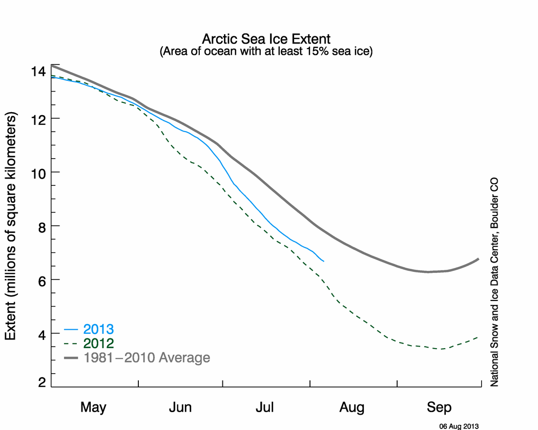
This is the latest the melt has ever been………..
Those lines are behaving like 2 similar poles of two magnets.
They want to repel each other.
NSIDC must have magnetized them when they made the changes.
National Sucker Institute Disseminating Crap.
Pixel counting the map will NOT give you the same answer as the “average” line on the chart.
The line on the chart represents the average of the summed pixels for 1979-2000. Pixel counting the map will give you the sum of the averaged pixels. This is not the same thing. I’ve already given a example for why they’re different: let me repeat if for the sake of clarity.
Exercise 1
Let’s pretend there are just two pixels on the map. If the concentration is above 15%, then it is included in the area. If below 15%, then it’s excluded.
Year 1: Pixel A = 100%, Pixel B = 10%.
Year 2: Pixel A = 10%, Pixel B = 100%.
What happens when we take the average? Well, it depends on the order of operations. If you count the pixels before averaging years, then both years have an extent of 1 pixel, and so the “average” extent is also 1 pixel. If you calculate the average concentration for each pixel before summing them, then both pixels have an average concentration of 55%, and so the “average” extent is 2 pixels. This means that if the ice edge consists of a mixture of very high/low concentration pixels, then the “map” method of averaging the pixels prior to summing them will tend to increase the calculated average ice extent.
Exercise 2:
Again, pretend there are just two pixels on the map.
Year 1: Pixel A = 19%, Pixel B = 10%.
Year 2: Pixel A = 10%, Pixel B = 19%.
What happens when we take the average in this case? Once again it depends on the order of operations. If you count pixels before averaging years, then both years have an extent of 1 pixel, and so the “average” extent is also 1 pixel. If you calculate the average concentration for each pixel before summing them, then both pixels have an average concentration of 14.5%, and so the “average” extent is 0 pixels. This means that if the ice edge consists of a mixture of pixels just below/above the 15% threshold, then the “map” method of averaging the pixels prior to summing them will tend to increase the calculated average ice extent.
Of the two possibilities, the second is closer to reality. Thus, it’s not particularly surprising that the average extent (calculated from the map) is lower than the average extent shown on the line graph. Pixel counting the map will NOT tell you whether this year’s line is about to cross the “average” line on the graph.


No ice loss in 23 years. What kind of “catastrophic warming” is that? Why isn’t the Washington Post reporting this important story?
If these alarmists had any sense of shame, they would come clean and admit they were wrong.
The one thing that global warming is supposed to do….amplified at the poles, and make spring come sooner….
This is the latest the melt has ever been………..
Those lines are behaving like 2 similar poles of two magnets.
They want to repel each other.
NSIDC must have magnetized them when they made the changes.
National Sucker Institute Disseminating Crap.
tick-tock, tick-tock…
NSIDC… I’m waiting….
tick-tock, tick-tock…
When are you going to catch up with the rest of the charts that show Arctic ice is above average.?
Their graph uses a smoothing/averaging algorithm…5-day moving average if I remember correctly. So give it a couple more days and see what happens.
-Scott
Pixel counting the map will NOT give you the same answer as the “average” line on the chart.
The line on the chart represents the average of the summed pixels for 1979-2000. Pixel counting the map will give you the sum of the averaged pixels. This is not the same thing. I’ve already given a example for why they’re different: let me repeat if for the sake of clarity.
Exercise 1
Let’s pretend there are just two pixels on the map. If the concentration is above 15%, then it is included in the area. If below 15%, then it’s excluded.
Year 1: Pixel A = 100%, Pixel B = 10%.
Year 2: Pixel A = 10%, Pixel B = 100%.
What happens when we take the average? Well, it depends on the order of operations. If you count the pixels before averaging years, then both years have an extent of 1 pixel, and so the “average” extent is also 1 pixel. If you calculate the average concentration for each pixel before summing them, then both pixels have an average concentration of 55%, and so the “average” extent is 2 pixels. This means that if the ice edge consists of a mixture of very high/low concentration pixels, then the “map” method of averaging the pixels prior to summing them will tend to increase the calculated average ice extent.
Exercise 2:
Again, pretend there are just two pixels on the map.
Year 1: Pixel A = 19%, Pixel B = 10%.
Year 2: Pixel A = 10%, Pixel B = 19%.
What happens when we take the average in this case? Once again it depends on the order of operations. If you count pixels before averaging years, then both years have an extent of 1 pixel, and so the “average” extent is also 1 pixel. If you calculate the average concentration for each pixel before summing them, then both pixels have an average concentration of 14.5%, and so the “average” extent is 0 pixels. This means that if the ice edge consists of a mixture of pixels just below/above the 15% threshold, then the “map” method of averaging the pixels prior to summing them will tend to increase the calculated average ice extent.
Of the two possibilities, the second is closer to reality. Thus, it’s not particularly surprising that the average extent (calculated from the map) is lower than the average extent shown on the line graph. Pixel counting the map will NOT tell you whether this year’s line is about to cross the “average” line on the graph.